Examples provided here are purely for illustrating software features and functionality.

Weibull++ Example 4 – Degradation Analysis Example

Download Example File for Version 10 (*.rsgz10) or Version 9 (*.rsr9)

Background

Five turbine blades were tested for crack propagation. The test units were cyclically stressed and inspected every 100,000 cycles for crack length. Failure is defined as a crack of length 30 mm or greater.

Using Weibull++’s degradation analysis folio and Quick Calculation Pad (QCP), determine the B10 life for the blades using degradation analysiswith an exponential model for the extrapolation.

Experiment and Data

The following table shows the test results for the five units at each cycle.

Cycle (x100)	Unit A	Unit B	Unit C	Unit D	Unit E
100	15 mm	10 mm	17 mm	12 mm	10 mm
200	20 mm	15 mm	25 mm	16 mm	15 mm
300	22 mm	20 mm	26 mm	17 mm	20 mm
400	26 mm	25 mm	27 mm	20 mm	26 mm
500	29 mm	30 mm	33 mm	26 mm	33 mm

Analysis

Step 1: Using Weibull++, create a degradation analysis folio and enter the data into the data sheet. Select Exponential for the model and enter 30 for the critical degradation level. These settings will be used to extrapolate a failure time for each unit. To specify how the failure times will be analyzed, select 2P-Weibull for the life distribution and select MLE for the analysis method. After you calculate the folio, it will appear as shown next.

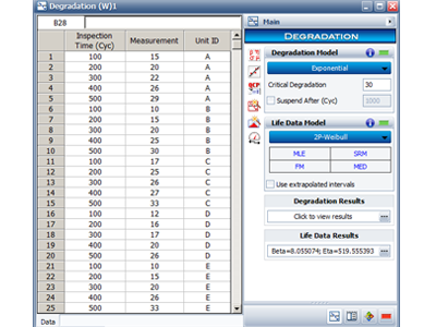
Figure 1: Degradation folio with data and results.

To view the parameters of the degradation model, click anywhere inside the Degradation Results area. The parameters will appear in the Results window, as shown next. (The second tab of the Results window shows the failure times that were extrapolated from the model.)

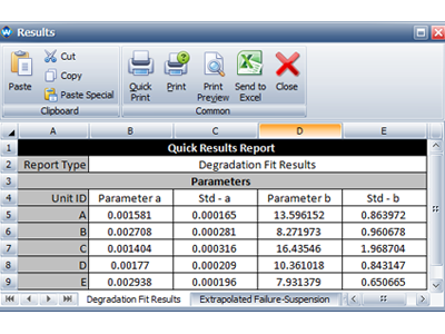
Figure 2: Results window showing the parameters of the degradation model.

Step 2: Next, view the linear Degradation vs. Time plot for the degradation analysis, as shown next. This plot shows how each unit degraded over time, and the horizontal pink line indicates the level at which a unit is considered failed.

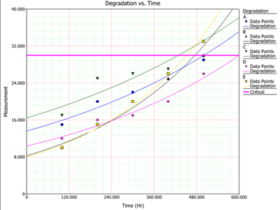
Figure 3: Degradation vs. Time (Linear) plot.

Step 3: Return to the data sheet, and then view the results of the life data analysis on the extrapolated failure times by clicking anywhere inside the Life Data Results area.

Figure 4: Results of life data analysis on the extrapolated failure times.

Step 4: Using the QCP, the B10 life is calculated to be 392.9179 (x100) cycles, as shown next.

Figure 5: Using the QCP to calculate the B10 life.