

 Our mission is to lead innovation by providing the most advanced solutions in reliability and sustainability to empower…
 REC is looking to the future by aligning business goals with Saudi Arabia’s 2030 Vision. Part of this is investing in our young people and their future.
 Reliability Expert Center was established with the strategic vision of spreading a reliability and sustainability culture across Saudi Arabia.


Download Example File for Version 10 (*.rsgz10) or Version 9 (*.rsr9)
This example shows you how to use allocation analysis to improve the reliability of a system by improving the reliability of its individual components.
Figure 1: System RBD
Subsystem A can be broken down into two assemblies, A and B, as shown next.
Figure 2: RBD of Subsystem A
Subsystem B can also be broken down into two assemblies, C and D.
Figure 3: RBD of Subsystem B
Figure 4: RBD of Assembly A
Figure 5: RBD of Assembly B
Figure 6: RBD of Assembly C
Figure 7: RBD of Assembly D
| Component | Life (Failure) Distribution | ||
| Comp. 1 | Weibull | Beta = 2 | Eta = 5,000 hours |
| Comp. 2 | Weibull | Beta = 2 | Eta = 4,500 hours |
| Comp. 3 | Weibull | Beta = 1.5 | Eta = 8,965 hours |
| Comp. 4 | Weibull | Beta = 1 | Eta = 8,000 hours |
| Comp. 5 | Lognormal | Log Mean = 10 hours | Log Std = 1.4 hours |
| Comp. 6 | Weibull | Beta = 3 | Eta = 10,000 hours |
| Comp. 7 | Weibull | Beta = 3 | Eta = 6,000 hours |
| Comp. 8 | Exponential | Mean = 10,000 hours | – |
| Comp. 9 | Weibull | Beta = 2.2 | Eta = 7,000 hours |
Step 1: Estimate the system reliability of the configuration at 500 hours. The following picture shows that the estimated reliability is 92.56565%, as calculated in BlockSim.
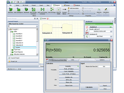
Figure 8: System Reliability Calculated Using BlockSim
where:
We’ll set Subsystem A to f = 0.9 and Subsystem B to f = 0.7. The Rmax for both subsystems is 99.999% at 500 hours.
The optimum allocation scheme for each subsystem is the one that satisfies:
Solving this yields an optimum allocation for each subsystem. The solution can also be obtained via the allocation analysis tool in BlockSim.
BlockSim allows you to use a predefined feasibility value in the calculation. You select the value from a set shown on a scale from Easy (1) to Hard (9). The relationship between the scale values (SV) in BlockSim to the feasibility function in Eqn. (1) is described as:
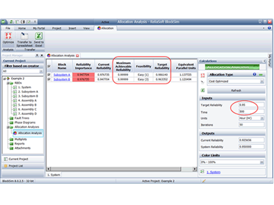
Figure 9: Allocation Analysis Tool in BlockSim.
| Feasibility (SV) | Target R, 500 hrs | |
| System | 0.95 | |
| Subsystem A | 1 | 0.986140 |
| Assembly A | 1 | 0.987318 |
| Comp. 1 | 1 | 0.997046 |
| Comp. 2 | 9 | 0.990243 |
| Assembly B | 9 | 0.979923 |
| Comp. 3 | 1 | 0.986916 |
| Comp. 4 | 1 | 0.939413 |
| Comp. 5 | 1 | 0.996573 |
| Subsystem B | 3 | 0.963352 |
| Assembly C | 9 | 0.999297 |
| Comp. 6 | 1 | 0.999875 |
| Comp. 7 | 1 | 0.999422 |
| Assembly D | 1 | 0.964030 |
| Comp. 8 | 1 | 0.966936 |
| Comp. 9 | 1 | 0.996995 |
